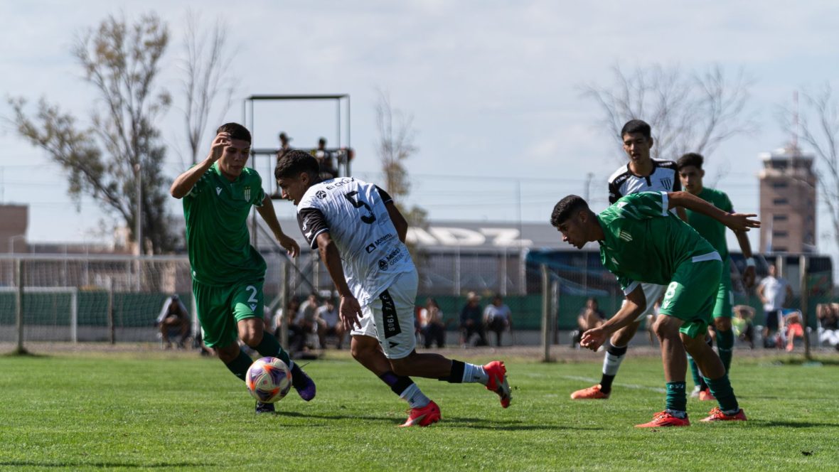
Predictability lives in the match log, not the headline figure.
Consider two teams across five matches. Team A records 5, 6, 6, 6 and 7 corners; Team B records 1, 3, 6, 9 and 11. Both average six, but Team A repeatedly finishes near that figure. Team B’s mean is held together by extremes, so six poorly represents its usual output.
Top Free Bets for October
BetUS
200% up to $1,000
18+. Full T&C's apply. Sports bonus: 100% match up to $500. Casino bonus: 100% match up to $500. Enter promo code NEW200 at deposit and get up to a $1000 bonus. Valid on your first three (3) deposits. Available for all deposit methods. Minimum deposit of $50.
18+. Full terms apply. The Bet Back Bonus is available for new customers on first-time deposits of $50 or more. To redeem, select the offer in the cashier while completing your first deposit. Make your pick(s) in the Sportsbook and then select ‘Opt In to Use Your Bonus’. A Bet Back Bonus pop-up will display, select ‘Claim’ and then enter the risk amount to place your bet. If it wins, you keep your profits. If it loses, get 100% of your risk refunded as Free Play with only 1-time rollover. Free Play can then be used to place bets in the Sportsbook and earn cash. Additional T&Cs apply, please visit MyBookie to access the Help Center or contact Live Chat for more details.
18+. Full T&C's apply. This promotion is available only to new accounts in North America. Freeplay amount must be wagered five times (5x rollover) before it becomes eligible for withdrawal. Only prematch (sportsbook) bets count toward the 5x rollover requirement. Each person may claim only one bonus. If a customer creates multiple accounts to exploit this promotion, bet105 will mark all related accounts as ineligible and reclaim the funds. If a client receives more than two free bets without making a deposit, any winnings from those bets will be forfeited. This promotion applies only to the initial deposit or if specifically assigned by bet105.
18+. Full terms apply. New BUSR members only. Minimum deposit of $50 required per qualifying deposits. Codes 300SB1, 300SB2, and 300SB3 must be entered at the time of each corresponding deposit.
Each code is valid one time only. Each bonus code must be claimed at least 24 hours apart. Only one promo code may be applied per deposit. A 20x rollover requirement applies to the combined total of your initial deposit and bonus before any withdrawal can be made. Redeemable in the Sportsbook only. BUSR management reserves the right to modify, suspend, or cancel this promotion at any time. Redeem each promo code in the cashier to get your bonus. Must be 18 or older. Please gamble responsibly. General House Rules Apply.
18+. Full terms apply. 100% up to $500 Bonus. Valid for non-crypto payment methods only. Minimum deposit amount $50. This offer is not available to customers from Canada or Mexico. The bonus code must be redeemed immediately after the deposit and before a wager has been placed. The sum of the deposit and the bonus are subject to rollover requirements of 12x at min. odds of -200 (1.5) before a new code can be redeemed. Max. $500 of each bet count towards the rollover requirements. Only bets placed on options that take place count towards the rollover requirements. Wagers on Horse Racing and Boosted Odds do not count towards the rollover requirements. All general Everygame Sportsbook rules apply.
21+. Full T&C's apply. Bonus: 35% of qualifying deposit, up to $105. Rollover: 8× (only sports action counts towards the rollover) deposit + bonus. Expiry: 7 days after credit. Hold period: 2 weeks. Payouts allowed only after rollover and hold period are completed. Example: Deposit $200 → Receive $50 Sports Free Play. Sports Free Play Rules: see the BetAnything General Reward Rules for eligible sports, wager types, odds, and rollover rules.
18+. Full T&C's apply. This bonus can only be redeemed on your first deposit. Rollover is 5x Sports/5x Horses/30x Casino on both the initial deposit and the bonus amount. Rollover in our Sportsbook, for winning wagers, will be determined by the lesser of your risk or win amount at the time of wager settlement; for losing wagers your risk amount will be credited to your rollover contribution. Bonus funds cannot be used for play on Live Dealer games. Live Dealer play does not count toward meeting Casino rollover requirements for withdrawal. If a withdrawal is made before the bonus terms are met, all bonus funds as well as any money earned by wagering the bonus will be forfeited.
Consistency rests on spread and repeatability. A quick range check gives Team A a spread of two corners, compared with ten for Team B. It also helps to count results within a practical band: Team A lands between five and seven in all five matches, while Team B does so only once. No pattern guarantees the next result, but a tight cluster provides stronger evidence of stable corner production than the mean alone.
Define the numbers before comparing teams
Three corner figures answer different questions:
Corners won measure how often a team earns corners through its own attacks.
Corners conceded measure how many opponents earn against that team.
Total match corners combine both sides’ corners. A high total may reflect attacking pressure, defensive vulnerability, or both.
For example, a team averaging six corners won and five conceded produces an 11-corner match average. That does not make it equally consistent in each measure. The distributions must be checked separately, as explained in the broader guide to interpreting corner statistics.
Before calculating averages, ranges, or hit rates, fix three conditions: sample length, competition, and data source. Comparing one club’s last five league matches with another club’s last ten matches across all competitions creates avoidable noise. Cup games, extra time, and inconsistent provider corrections can distort the result.
A practical baseline is the same number of recent league matches from one provider, with extra-time corners excluded. Record the date range so the comparison can be reproduced later.
Build a fixture-level baseline
Create one row per fixture before calculating team-level figures. Useful columns include date, opponent, venue, corners won, corners conceded, and total corners. Keeping the raw match rows makes unusual results easy to spot and allows later filtering by home, away, or competition.
Consider five total-corner results:
Fixture
Total corners
1
8
2
9
3
9
4
10
5
24
The mean is (8 + 9 + 9 + 10 + 24) ÷ 5 = 12. It remains a useful baseline because it captures the full corner volume across the sample.
The median is the middle value after sorting the results, so it is 9. That figure better represents a typical fixture because the 24-corner match pulls the mean upward without affecting the center of the distribution.
Neither measure should replace the other. A wide gap between mean and median flags possible distortion and provides a reason to inspect the extreme fixture. For an even number of matches, the median is the average of the two middle values.
Worked comparison
Measure how tightly results cluster
Consider two teams’ total corners across eight comparable fixtures:
Team
Match totals
Mean
Range
IQR
Standard deviation
MAD
A
9, 10, 10, 10, 10, 10, 10, 11
10
2
0
0.50
0.25
B
4, 6, 8, 9, 11, 12, 14, 16
10
12
6
3.78
3.25
Both teams average 10 corners, but their distributions tell different stories. Range compares the lowest and highest values, so it quickly shows that Team B swings much more widely. However, one unusual fixture can distort it.
Interquartile range (IQR) measures the middle half of the results. Team A’s IQR of 0 means its central four values are identical, while Team B’s middle results still cover six corners. This makes IQR useful when occasional extremes are present.
Standard deviation gives greater weight to results far from the mean. Team B’s large misses in both directions therefore raise its figure sharply. The values shown use population standard deviation; some spreadsheets default to the sample version.
Mean absolute deviation (MAD) averages each result’s distance from the mean. It is often the easiest measure to interpret: Team A typically sits only 0.25 corners from its average, compared with 3.25 for Team B.
Check comparability first
Lower spread supports a consistency claim only when teams have similar averages, equal or reasonably close sample sizes, and comparable fixtures. A low spread around six corners is not equivalent to a low spread around ten.
Targeted consistency
Test consistency around the target
Use bands and hit rates to measure repeatability where it matters.
Dispersion measures describe overall statistical stability, but the practical question often concerns a particular result range or line. A team consistently producing seven corners may be highly stable, yet offer little support for a target of ten or more.
Measure band frequency
A band hit rate is the percentage of fixtures finishing inside a defined range:
Fixtures inside the band ÷ total fixtures × 100
Suppose a team’s total-corner results are 9, 10, 11, 10, and 14. Four of five fixtures fall within the 9–11 band, giving an 80% hit rate. The result of 14 increases dispersion, but the band still reveals a strong tendency to land near the desired zone.
Check the exact threshold
Threshold rates answer a narrower question: how often did the result clear the relevant line? In the same sample:
Over 9.5 corners: 4 of 5 fixtures, or 80%
Over 10.5 corners: 2 of 5 fixtures, or 40%
That one-corner shift changes the conclusion substantially. Bands are most useful for identifying a repeatable result area; thresholds test whether that pattern actually satisfies a chosen cutoff.
Set bands and lines before reviewing the data, and compare identical home, away, competition, and sample conditions. Otherwise, a convenient boundary can make ordinary results appear unusually consistent.
Sample check
Test recent form against a longer window
A five-match run can flag a change, but it should be placed beside the team’s rolling 10- and 15-match figures. Compare the same measures—mean, median, spread, band frequency, and threshold rate—across all three windows.
Similar results across windows: the pattern appears more durable.
Strong five-match improvement only: treat it as a possible streak.
A gradual shift across every window: confidence in a genuine change increases.
Check where the windows cross a managerial appointment, tactical switch, key injury, promotion, relegation, or unusually difficult schedule. A clear structural break may justify starting a fresh baseline. Otherwise, retain the larger sample and use recent matches as supporting evidence rather than allowing them to replace it.
Watch the fixture mix
Five matches against corner-heavy opponents can distort recent form. Note opponent strength and home-away balance before treating the change as meaningful.
Stress-test the pattern by context
Separate venue effects from opponent-driven patterns
An overall corner record can look remarkably steady while combining two very different profiles. A team averaging 5.8 corners across 20 fixtures might produce a tight 6–7 range at home but swing between 2 and 8 away. The first check should therefore compare consistency across home and away fixtures, not merely compare their averages.
For each venue split, recalculate the median, IQR, band frequency, and threshold rate. Keep sample sizes visible: eight stable home matches carry less weight than 25 spread across several months.
Add opponent context
Broad groupings can reveal where the pattern survives:
Strength: top, middle, and bottom thirds of the table.
Possession style: dominant-possession sides versus teams comfortable without the ball.
Defensive shape: low-block opponents versus teams that press or defend higher.
Groups should be defined consistently, preferably using information available before each match rather than final league positions. Avoid slicing too finely; tiny categories can manufacture apparent patterns.
The final claim should match the evidence. “Consistent at home against mid- and lower-table opponents” is more useful—and more defensible—than calling the team consistent in every setting.
Pattern check
Find the source of stable totals
Separate repeatable pressure from opponent-driven noise
A stable match total can hide different engines. One team may win corners through sustained territory, repeated crosses, and blocked shots; another may reach similar totals because it spends long periods defending. When both patterns are steady, total corners are usually more dependable.
The source becomes clearer when fixture-level corners won and conceded are examined separately. The assessment should balance corners generated with corners allowed, then check how much each side varies:
Attacking pressure: corners won remain tightly grouped across matches and contexts.
Defensive pressure: corners conceded repeatedly sit within a narrow band.
Two-way stability: both measures cluster, supporting a stable combined total.
Opponent contributions can still break the pattern. A team might reliably win six corners, but total-match results will swing if opponents contribute anywhere from one to eight. This is especially important when consistency appears in the team’s own count but not in the combined total.
A practical assessment combines the median, dispersion, band frequency, recent-window agreement, venue splits, and the separate stability of corners won and conceded. Confidence is stronger when several signals point in the same direction and no single outlier drives the result. Only after that evidence is assembled should the market line and price determine whether the pattern offers enough margin.
Key Takeaways
Identify the engineStable totals may come from attack, defence, or both.
Check opponent noiseWide variation in opponent corners weakens total-match reliability.
Combine the signalsRequire agreement across several stability measures before considering price.
Final check
Keep only patterns that hold up
Require a comparable sample
Use enough fixtures to reduce one-off effects, with the same competition, metric, and data source throughout.
Seek agreement between signals
Retain teams only when low variation, a tight result band, and strong target hit rates point in the same direction.
Recheck the context
Confirm that venue, opponent strength, and attacking-versus-defensive splits do not explain away the pattern.
Discount fragile evidence
Treat small samples and isolated winning streaks as provisional, however impressive the headline rate appears.
There is no universal consistency cutoff. A credible candidate combines stable match-level results with a strong hit rate across a sufficiently broad, comparable sample—and remains convincing after practical context checks.
Top Free Bets for October
BetUS
200% up to $1,000
18+. Full T&C's apply. Sports bonus: 100% match up to $500. Casino bonus: 100% match up to $500. Enter promo code NEW200 at deposit and get up to a $1000 bonus. Valid on your first three (3) deposits. Available for all deposit methods. Minimum deposit of $50.
18+. Full terms apply. The Bet Back Bonus is available for new customers on first-time deposits of $50 or more. To redeem, select the offer in the cashier while completing your first deposit. Make your pick(s) in the Sportsbook and then select ‘Opt In to Use Your Bonus’. A Bet Back Bonus pop-up will display, select ‘Claim’ and then enter the risk amount to place your bet. If it wins, you keep your profits. If it loses, get 100% of your risk refunded as Free Play with only 1-time rollover. Free Play can then be used to place bets in the Sportsbook and earn cash. Additional T&Cs apply, please visit MyBookie to access the Help Center or contact Live Chat for more details.
18+. Full T&C's apply. This promotion is available only to new accounts in North America. Freeplay amount must be wagered five times (5x rollover) before it becomes eligible for withdrawal. Only prematch (sportsbook) bets count toward the 5x rollover requirement. Each person may claim only one bonus. If a customer creates multiple accounts to exploit this promotion, bet105 will mark all related accounts as ineligible and reclaim the funds. If a client receives more than two free bets without making a deposit, any winnings from those bets will be forfeited. This promotion applies only to the initial deposit or if specifically assigned by bet105.
18+. Full terms apply. New BUSR members only. Minimum deposit of $50 required per qualifying deposits. Codes 300SB1, 300SB2, and 300SB3 must be entered at the time of each corresponding deposit.
Each code is valid one time only. Each bonus code must be claimed at least 24 hours apart. Only one promo code may be applied per deposit. A 20x rollover requirement applies to the combined total of your initial deposit and bonus before any withdrawal can be made. Redeemable in the Sportsbook only. BUSR management reserves the right to modify, suspend, or cancel this promotion at any time. Redeem each promo code in the cashier to get your bonus. Must be 18 or older. Please gamble responsibly. General House Rules Apply.
18+. Full terms apply. 100% up to $500 Bonus. Valid for non-crypto payment methods only. Minimum deposit amount $50. This offer is not available to customers from Canada or Mexico. The bonus code must be redeemed immediately after the deposit and before a wager has been placed. The sum of the deposit and the bonus are subject to rollover requirements of 12x at min. odds of -200 (1.5) before a new code can be redeemed. Max. $500 of each bet count towards the rollover requirements. Only bets placed on options that take place count towards the rollover requirements. Wagers on Horse Racing and Boosted Odds do not count towards the rollover requirements. All general Everygame Sportsbook rules apply.
21+. Full T&C's apply. Bonus: 35% of qualifying deposit, up to $105. Rollover: 8× (only sports action counts towards the rollover) deposit + bonus. Expiry: 7 days after credit. Hold period: 2 weeks. Payouts allowed only after rollover and hold period are completed. Example: Deposit $200 → Receive $50 Sports Free Play. Sports Free Play Rules: see the BetAnything General Reward Rules for eligible sports, wager types, odds, and rollover rules.
18+. Full T&C's apply. This bonus can only be redeemed on your first deposit. Rollover is 5x Sports/5x Horses/30x Casino on both the initial deposit and the bonus amount. Rollover in our Sportsbook, for winning wagers, will be determined by the lesser of your risk or win amount at the time of wager settlement; for losing wagers your risk amount will be credited to your rollover contribution. Bonus funds cannot be used for play on Live Dealer games. Live Dealer play does not count toward meeting Casino rollover requirements for withdrawal. If a withdrawal is made before the bonus terms are met, all bonus funds as well as any money earned by wagering the bonus will be forfeited.
Hi I'm Andy and I love to report on the latest football scores and Tables. I also like to have a bet on the football and occasionaly on the horses. On this website I have new bookmaker offers listed that will give you free bets and bonuses to help you beat the bookies. Enjoy your stay.